

~ 5 min read
How does a Linear Regression model work?

Nizar Haider
While LR may be the simplest machine learning model out there a lot of us don't know much about what happens under the hood. In this article you will learn:
- How LR calculates the line of best fit
- Regression evaluation metrics (MAE, MSE and R2)
- Optimization technique using gradient descent
- Some assumptions of using LR
What is Linear Regression?
It's a statistical technique that models the relationship between 2 or more variables whose output is continous. It falls under the supervised regression class of machine learning. Some examples of its application are:
- Predicting what the score of a student would be on an exam (20, 39, etc...)
- Predicting the number of tourists visitng Sri Lanka monthly (122,132, 353,239, ...)
Simple LR Model
Let's break down the simple LR model into 3 main parts and then analyse each of them.
- Calculating the line of best fit
- Optimization
- Evaluation of model
1. Calculating the line of best fit
Now the equation y = mx + c may be familiar to many of you and although a little different, it is the same equation in function for Simple Linear Regression.
Here is the equation for a simple LR model, statistically known as the simple regression model formula:
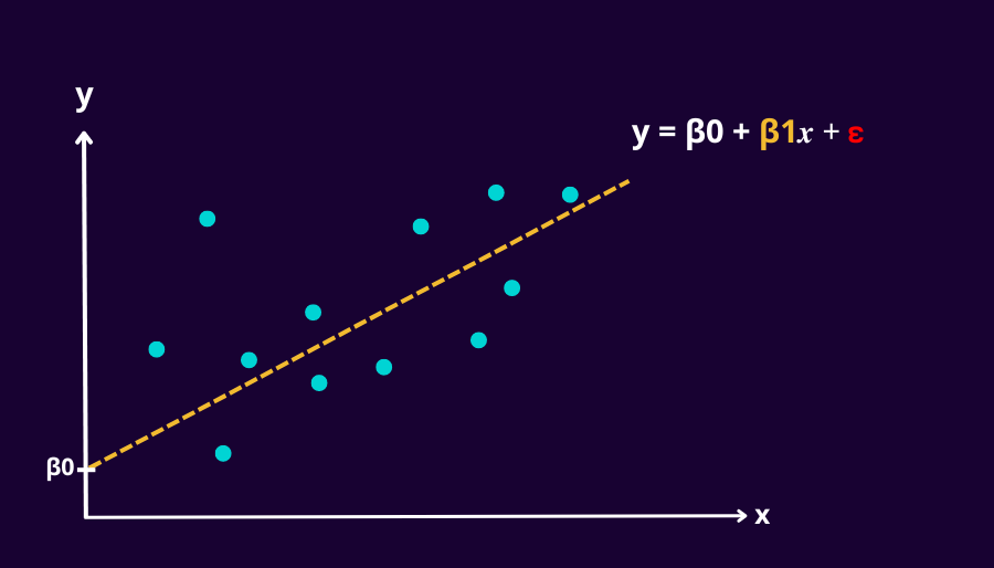

Sometimes you may notice the extra error term, ε (excluded in the simple regression model equation currently). The error term includes everything that separates your model predictions from the whole population. This means that it will reflect nonlinearities, unpredictable effects, measurement errors, and omitted variables. This is different from residuals which is the difference between your models predictions and a sample of the population.
Another way of putting it is in the sample we only consider one independant variable while in the population we consider all affecting factors.
However, the error term and residuals are interchanged a lot on the internet which can lead to some confusion. This article explains the distinction pretty well.
1.1 Calculating β1

Simply, β1 is just the covariance of (x,y) over the variation of x. In other words its the degree to which two variables (𝒙, y) change together over how spread out the data points of 𝒙 is.
Alternatively, here is another way of showing the equation:

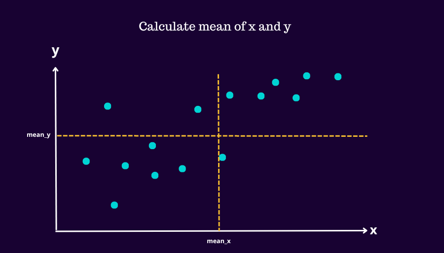
We get the mean values of x and y
Then we calculate the slope
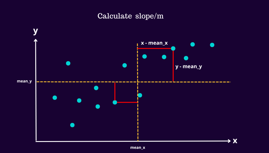
- xi is a value of x at index i.
- yi is a value of y at index i.
- x̅ is the mean of x.
- y̅ is the mean of y.
Now that we finally have our β1. We can move on to the other part of the equation.
1.2 Estimating the intercept
The estimate of the intercept β0 should be easier to understand than the estimate of the coefficient β1.

- x̅ is mean of x.
- y̅ mean of y.
- β1 is the coefficient that I estimated from earlier.
The reason for using the mean of x and y to find the intercept is because the line of best fit is known to pass through it.
Now that we have know what β1 and β0 is we can plot the line of best fit!
2. Optimization
We will be using gradient descent as the optimizer for this case so let's break it down.
Gradient descent helps us find the minima of a our error function which in this case is going to be the MSE (you can also use custom error functions :). It finds the minima through iterations of calculations that involve finding the gradient through partial derivatives to know which way to move. The two main components of this algorithm are:
- Partially deriving our cost/error function which is MSE
- The learning rate which is usually set to around 0.001 to start
Since MSE is
(y - (mx + b))2
Our cost function, MSE, has two parts, m and b Let's first take a look at their partial derivations
After using the power and chain rule we get the partial derivation of m and b:
To see the full working watch this video
After running the gradient descent optimizer algorithm over a few thousand different iterations of m and b you will see the MSE value reach a plateau like this:
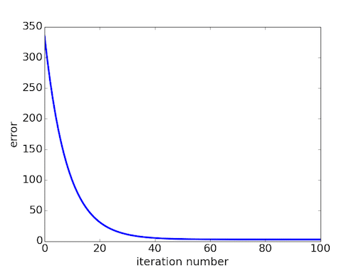
This means we have found the line of best fit!
3. Evaluation
How well does the independant variable, x explain the variance in dependant variable, y?
For this we use R2. The result is a value between 0 and 1, where 0 indicates that the model does not explain any variance, and 1 indicates a perfect fit where the model explains all the variance.
Mathematically represented as:
SSRESIDUAL: Squared sum difference between actual and predicted values SSTOTAL: Squared sum of difference between the actuals and the mean
There are a few more evaluation metrics you can check out:
- Mean Absolute Error (MAE)
- Mean Absolute Percentage Error (MAPE)
- Mean Percentage Error (MPE)
- Mean Square Error (MSE)
- Root Mean Squared Error (RMSE)
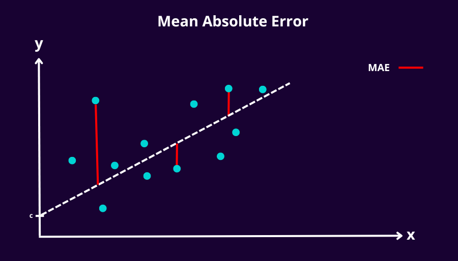
3.1 Mean Absolute Error
The mean absolute error (MAE) is the simplest regression error metric to understand. We just calculate the mean of sum of the differences between predicted and actual. Since the absolute of the values are taken they don't cancel each other out and so it gives us a way to evaluate the magnitutude of the residuals
Pros:
- Simplest evaluation and quickest to evaluate
Cons:
- Doesn't tell if the model is underperforming or overperforming since values are absolute
- Treats all magnitudes of residuals the same way
3.2 Mean Absolute Percentage Error
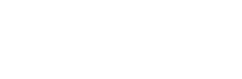
The mean absolute percentage error (MAPE) is a just MAE but quantified as a percentage. It just tells you how far your predictions are off from their corresponding actuals on average. Just like MAE it isn't affected by outliers.
Given it's division operation, it brings a couple weaknesses such as being undefined at data points that are equal to 0. It also is biased towards penalizing predictions that are over than actuals more than predictions that are under.
From the image below the MAPE is supposed to be 100% for both but they're not.
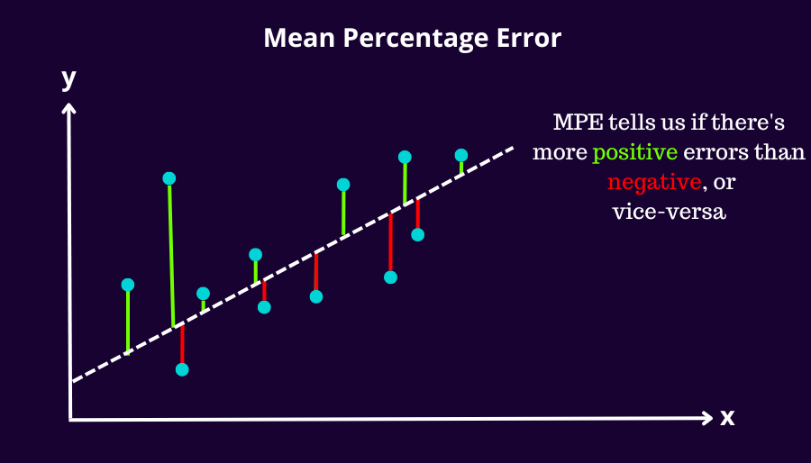
3.3 Mean Percentage Error

The mean percentage error (MPE) equation is exactly like that of MAPE. The only difference is that it lacks the absolute value operation. Due to this it's able to tell us about if the model is positively or negatively biased based on there being more negative residuals or vice versa respectively.
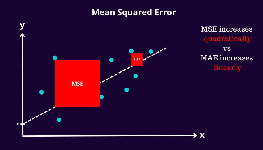
3.4 Mean Squared Error
The mean squared error (MSE) is the same as MAE except we square the residuals which adds robustness to outliers and penalize bigger residuals more than smaller ones. Therefore you cannot compare it to itself like you can with MAE but rather only against competing models.
Pros:
- More robust since it penalizes bigger residuals more
Cons:
- Values can get really large proving hard to read
- Can't be used to self-evaluate a model but rather its compeitiors
3.5 Root Mean Squared Error

The root mean squared error (RMSE) is a way researchers came up with to make MSE values smaller and more interpretable. It still maintains the benefits as MSE that includes dealing with outliers better. It's analogous to standard deviation in the sense that it measures how spread out the residuals are. Since its between 0 and 1, the lower the number the more accurate the model since there's less deviation and vice versa
It's also good practice to check MSE/MAE as well to get an idea of how well the predictions are doing along with the R2
Assumptions
Some assumptions we need to make of the data before using linear regression:
-
Linearity of Residuals: The independant variable(s) and dependant/target variable need to have a linear relationship
-
Independence of residuals: There should be no corelation between the residuals
-
Homoscedasticity: The variance of residuals should be the same across all independant variables which means they have to be spread out similarily. So like a random scatter on the horizontal line and no trend to be seen like widening or narrowing.
Notes
Remember how we had to first calculate the inital line of best fit for the LR model and then optimize it?
Well in machine learning scikit learn handles the initialization process and we can focus on the optimiztion aspect of it through hyper parameter tuning.
Next I'll be creating the model from scratch using scikit learn trying to predict how many tourists are going to visit Sri Lanka in the next month!