Building a Linear Regression Model from scratch

Regression is all about modelling the relationship between a dependant variable and its independant variable(s). Linear regression assumes that the relationship is linear and it's on this assumption that we can apply forecasting. Simple linear regression uses one indpendant variable while multiple linear regression uses 2 or more independant variables.

In this article we will be building a simple linear regression model from scratch on a jupyter notebook to model the relationship between tourist arrivals and exchange rate. Then we will compare it with the commonly used LR model from scikit learn library.

Some prerequisites include knowing:

• Sample regression formula
• Gradient Descent using MAE

If this seem alien to you then check this article out first on a complete breakdown of the linear regression model.

Not to worry I'll still give you a refresher.

The idea is to first decide on our error/cost function which is going to be MAE. The lower the MAE the better the model performs in terms of making predictions.

Now that we have the cost function, we should feed it into an optimizer like gradient descent and try to have the model converge on the optimal parameters to get the lowest MAE for the model.

1. Setup

---

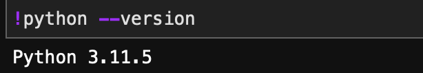
I'll be using a jupyter notebook for this with python version 3.11.

1.2 Dataset

Since we're trying to predict tourist arrivals in Sri Lanka we could use a few features to help us predict it.

• Exchange rate (USD to LKR)

Let's start with just using the exchange rate and see how well it does.

Here is the tail (last 5 rows) of the dataset:

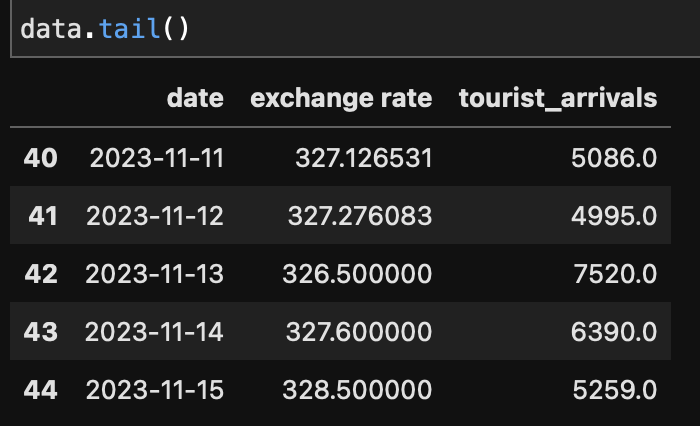
Now an important point to make here is the date column isn't needed. Since linear regression assumes that observations are independent of each other. Temporal data violates this assumption given their sequential order.

So we will proceed with just the exchange rate and tourist arrivals for now.

We will be importing just 3 libraries, Pandas, Matplotlib and Numpy

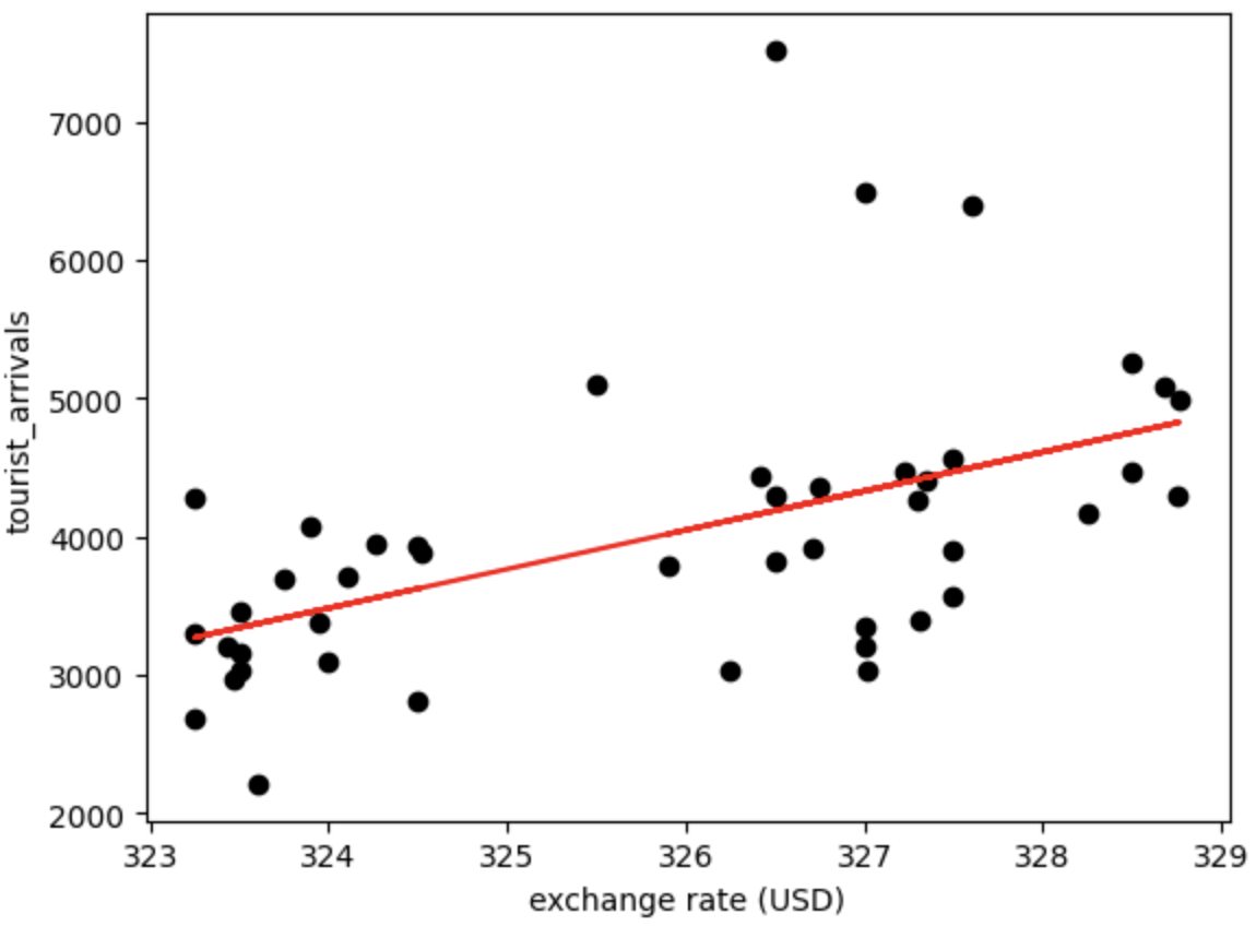
Let's take a look at a scatter plot of our features against each other.

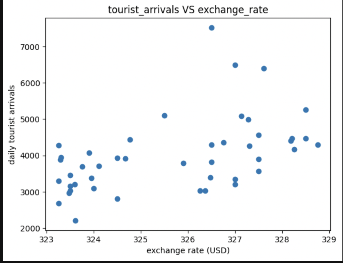
Here we see as the exchange rate increases there is an increase of tourist arrivals. A good test to do before attempting to model the relationship is to check for the variance of the features and make sure they are similar.

Variance of "tourist arrivals"

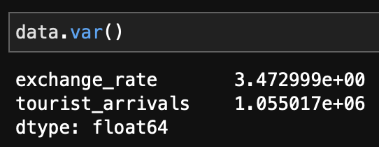
We can see that the tourist arrivals is a few order of magnitudes higher than the exchange rate. Hence we can apply techniques like normalizing or standardizing to fix this. I won't go into much detail on standardizing since this article is focused on building a linear regression model from scratch.

After standardizing it we can see the variance becomes 1 for both features and here is what the final plot looks like:

We can move on to the implementation of the code

2.Gradient Descent

To use gradient descent we need two components:

1. Cost/Loss function partials (to find out the gradients)
2. I just wanted to say 2 things, sounds cooler

2.1 Create gradient equation

Since we're using y - (mx + b) as the cost function we need to partially differentiate it. After doing so we get two partial equation for the parameters of m and b.

def gradient_descent(m_curr, b_curr, data, learning_rate):
    
    m_grad = 0
    b_grad = 0
    n = len(data)
    abs_error = 0
    
    for i in range(n):
        x = data_scaled[i][0]
        y = data_scaled[i][1]
        
        pred = (m_curr * x) + b_curr
        error = (y - pred)
        m_grad += -(2/n) * x * error
        b_grad += -(2/n) * error
        
        abs_error += abs(error)
    
    abs_mean_error = abs_error/n
    m =  m_curr - (m_grad * learning_rate)
    b =  b_curr - (b_grad * learning_rate)
    
    return abs_mean_error, m, b

Keep in mind using the dot product in numpy's library to find the sum of error is a better alternative than using a for loop.

2.2 Iterative Optimization

This function takes in the current value of m and b and is able to check the gradients of both m and b again and moves in the opposite direction to it.

learning_rate = 0.01
epochs = 500  
errors = []

#---Regression formula based initialization---
# m_scaled, b_scaled = initialization(data)

#---Random Initialization---
m_scaled = np.random.randn()  
b_scaled = np.random.randn()


for i in range(epochs):
            
    error, m_scaled, b_scaled = gradient_descent(m_scaled, b_scaled, data, learning_rate)
    
    if i % 10 == 0:
            print(f'Epoch: {i, error}')
    errors.append(error)

print(f'Final Coefficients: m={m_scaled}, b={b_scaled}')

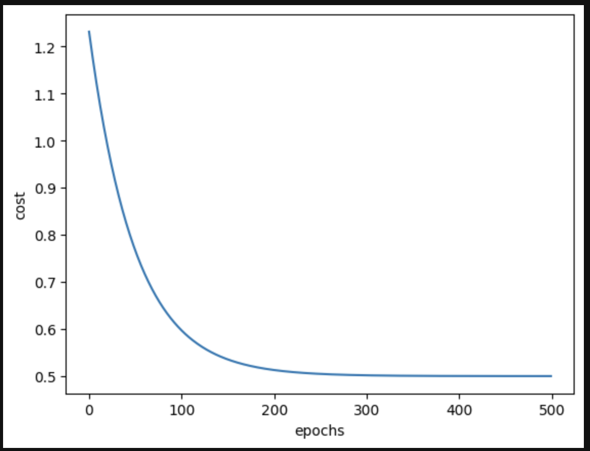
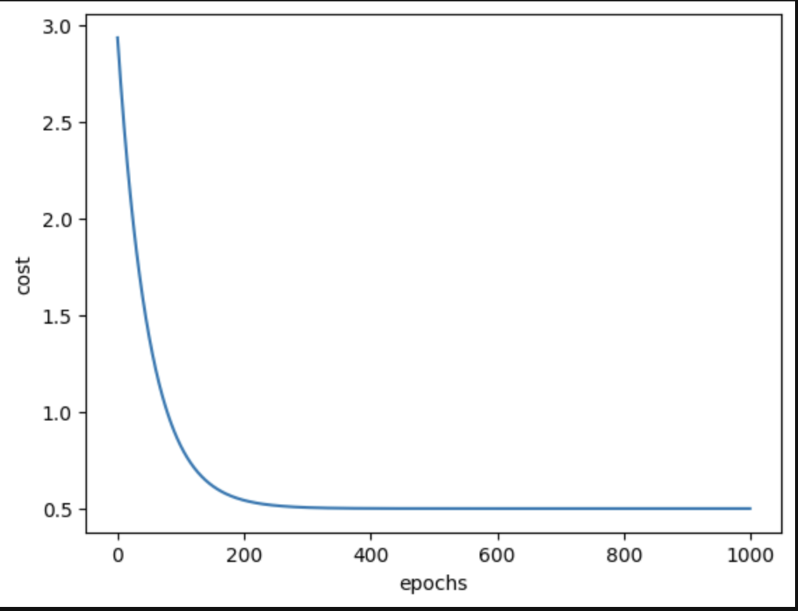
In this iterative optimization process you will see the cost value decrease as the algorithm converges on the minima for the parameters of m and b.

Optional (not really)

You can see here that we reach a kind of a plateau at around 300 epochs where the cost doesn't decrease significantly from there.

The number of iterations required involves mainly 2 things.

• Initial parameters of m and b
• Learning rate

If we initialize m and b using the linear regression formula

def initialization(data):
    x_mean = data.exchange_rate_scaled.mean()
    y_mean = data.tourist_arrivals_scaled.mean()
    cov_x_y = 0
    var_x = 0
    
    for i in range(len(data)):
        # x = data.iloc[i].exchange_rate_scaled
        # y = data.iloc[i].tourist_arrivals_scaled
        x = data_scaled[i][0]
        y = data_scaled[i][1]
        cov_x_y += ((x - x_mean)*(y - y_mean))
        var_x += (x - x_mean)**2 
        
    m = cov_x_y/var_x 
    b = y_mean - (beta * x_mean) 

    return m, b

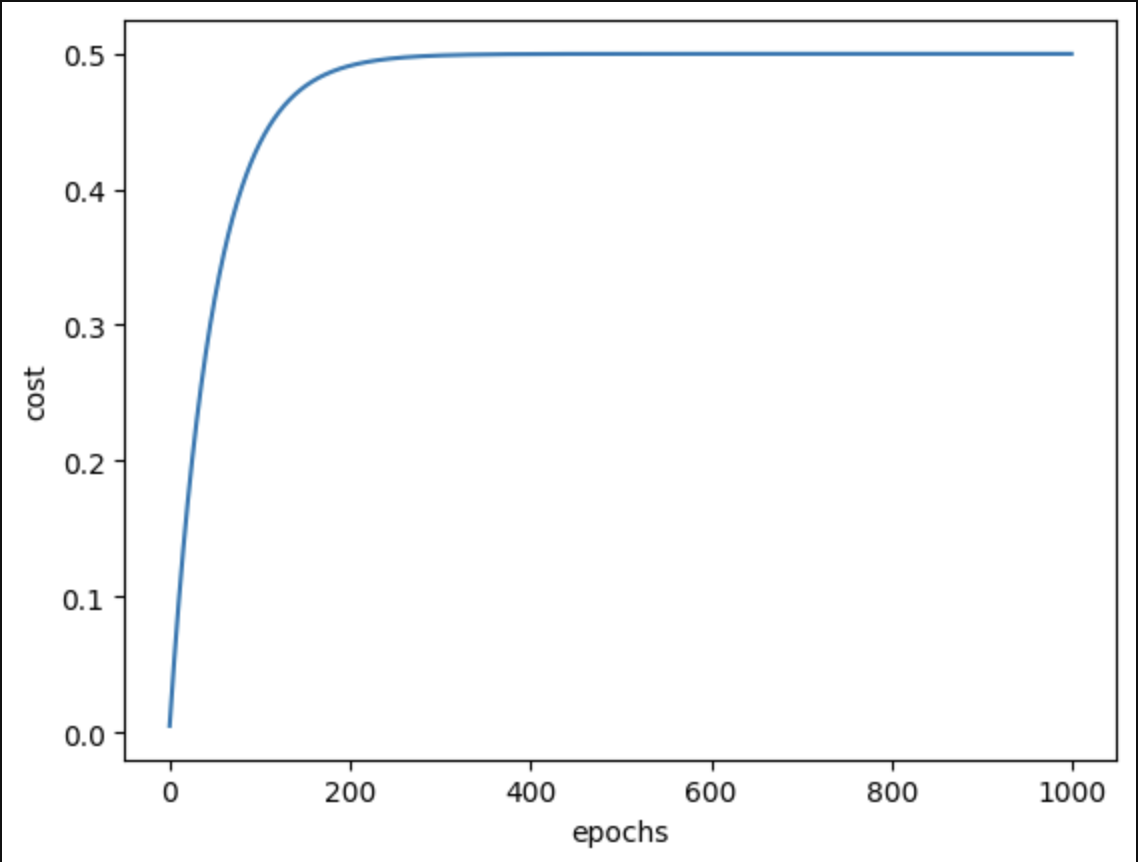
We wil see a major difference in the cost graph

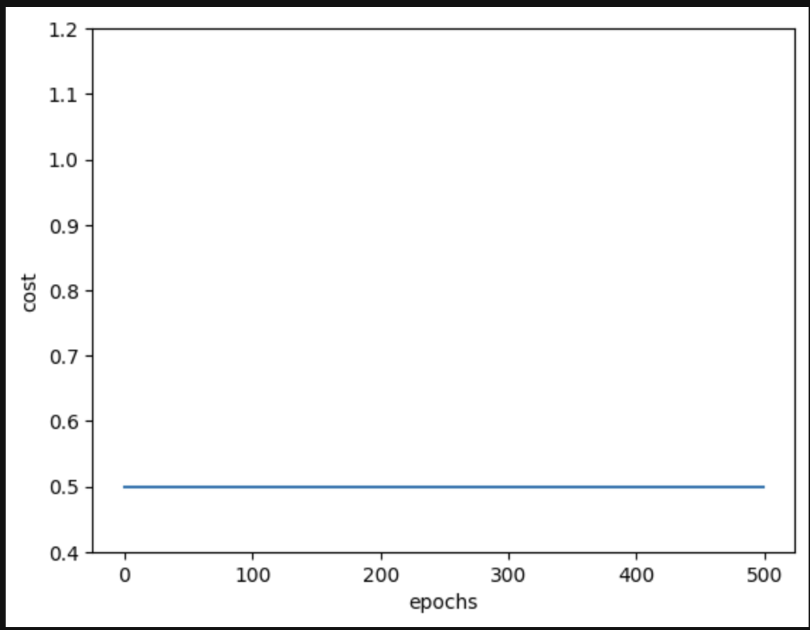
We can see that it reached relatively the same cost in only a matter of a few epochs compared to initializing the values as 0 and requireing over 300 epochs. However I dislike this method due to it being impractical and misleading at times. Some reasons i prefer randomly initializing a variable here is to make sure the model finds a global minima instead of a local one, also its also robust in handling a variety of data distributions, non-linear relationships, and outliers.

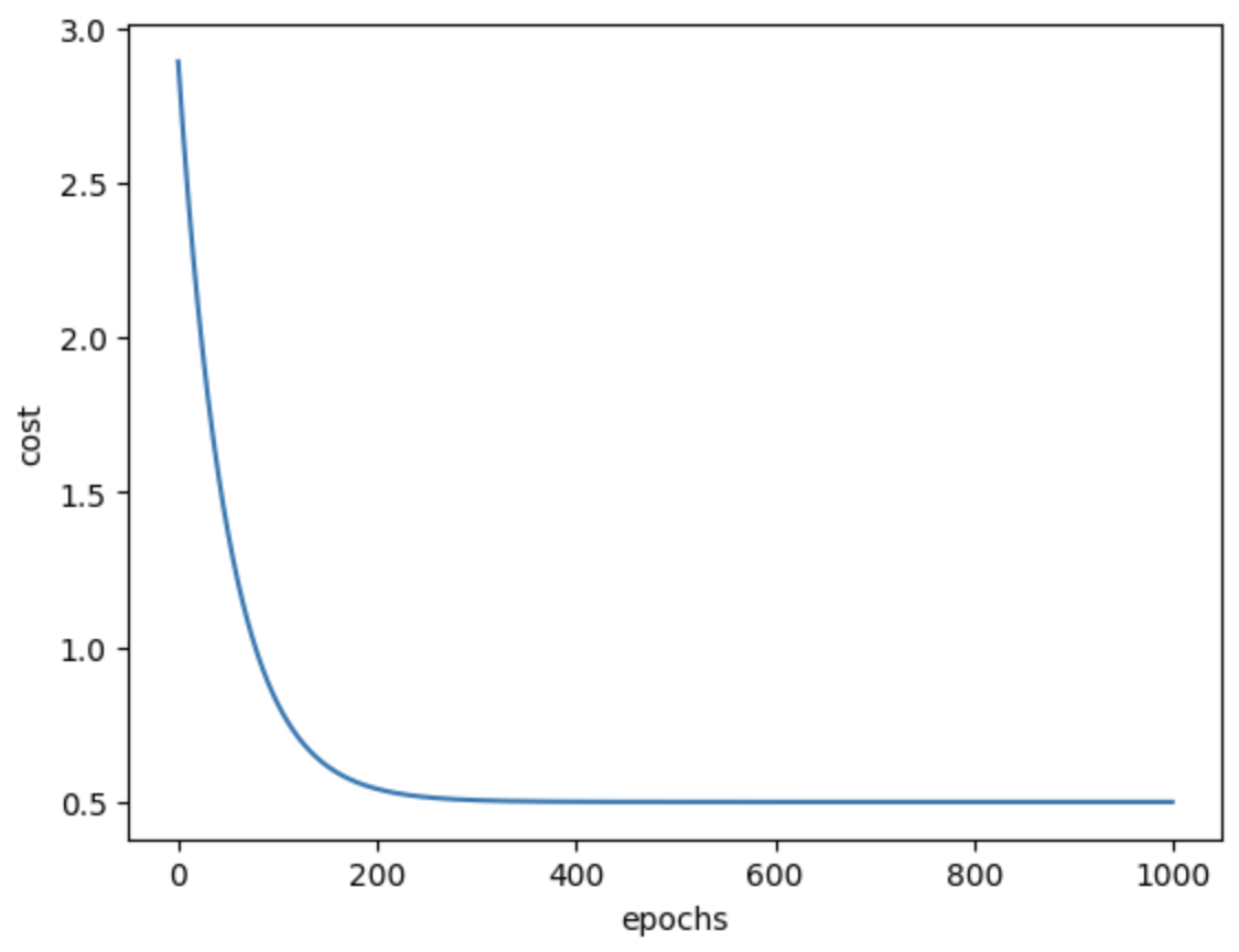
When you randomly initialize the values you should see it converge at the same value cost value for different values of m and b, this means you found the global variable. Here are some examples:

Example 1

Starting Cost: 2.892
Final cost: 0.499

Example 2

Starting Cost: 2.932
Final cost: 0.499

Example 3

Starting Cost: 0.005
Final cost: 0.499

So note always use random initialization!!! haha.

Here is what the final plot looks like

3.0 Comparison against Scikit Learn

For comparison here is the plot by importing a model from scikit learn

import numpy as np
import matplotlib.pyplot as plt
from sklearn.linear_model import LinearRegression

    
# Assuming you have a dataset X (features) and y (target variable)
# Replace X and y with your actual data

X = data.exchange_rate.values
y = data.tourist_arrivals

# Reshape X if it's a single feature
X = X.reshape(-1, 1)

# Create a Linear Regression model
model = LinearRegression()

# Fit the model to the data
model.fit(X, y)

# Get the coefficients (slope and intercept)
m = model.coef_[0]  # slope
b = model.intercept_  # intercept

# Generate points for the line
# x_line = np.linspace(min(X), max(X), 100).reshape(-1, 1)
y_line = model.predict(X)

# Plot the original data points
plt.scatter(X, y)

# Plot the linear regression line
plt.plot(X, y_line, color='red', label=f'y = {m:.2f}x + {b:.2f}')

# Label the axes
plt.xlabel('X')
plt.ylabel('y')

# Add a legend
plt.legend()

# Show the plot
plt.show()

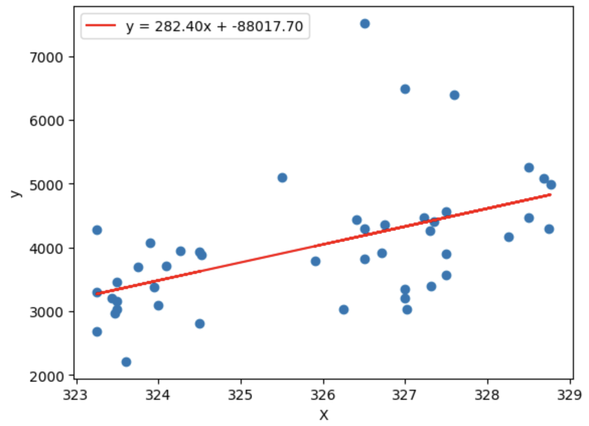
The plots are quite similar but looks can be deceiving (like my ex-wife) so let's take a look at the MAE scores:

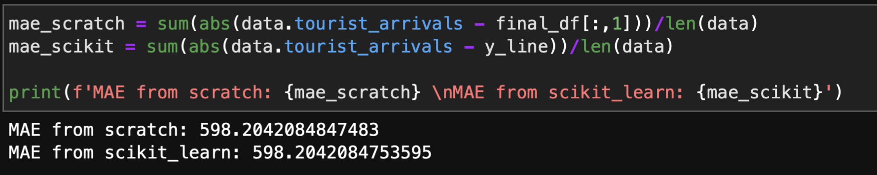
Our scores are pretty much the same and this tells us maybe my ex-wife wasn't all about looks after all.

We are done with the implementation of a linear regression model from scratch using python!

btw this model sucks at forecasting so don't use it lmao :)